Matching up to find the cause of loneliness

Aim

The Jean Golding Institute’s loneliness data challenge asks to investigate the relationship between the movement of people for education and loneliness. Our team set out to understand if there is significant evidence of the presence of causal relationships between loneliness and variables related to education and movement. We use matching to detect the presence of causal relationships between variables and demonstrate how it could be used to dismiss non-significant relationships that otherwise seem significant using basic statistical techniques.

Matching

Matching [1] is a method for designing experiments to discover causal effects, for example to assign patients to treatment and control groups in randomised control trials aimed at testing if a drug is effective. It can also be used for inferring the presence of causal relationships in observational studies where it is not possible to make interventions, for example when patients are free to decide whether or not to take the drug, provided that we can observe all the variables (covariates) that influence both the causal variable (taking the drug) and the outcome variable (recovery).

The general idea behind matching is to consider pairs of subjects that are similar in every aspect except for the value of the causal variable and determine if any difference observed in the value of the outcome variable is significant. For example, to find out if there is a causal relationship between the presence of schools close to a GP (causal variable) and loneliness (outcome variable) we proceed as follows:

1. Transform the causal variable, that in general can be discrete or continuous, into a binary variable. To this end, we assign the value 1 to all GPs where the number of schools (standardised) is larger than the median and 0 to all other GPs.

2. Consider all variables in our datasets that may affect the causal and the outcome variables. These variables are called confounders and those we consider in our study are listed in the Table below.

   Variable	Definition	Data source
   Number of nearby schools (z-score)	z-score of the total number of schools in the postcodes within 10km of the GP’s postcode	GOV.UK
   Multiple deprivation index	the official measure of relative deprivation for small areas in England	Provided by the Office of National Statistics
   Incoming migrants per capita (z-score)	z-score of the total number of incoming migrants in the GP’s local authority divided by the resident population	ONS
   Rural-urban index	Category defining the urbanisation of an area.	Provided by the Office of National Statistics
   Fraction of patients 0-9	percentage of the GP patients with age 0-9	NHS Digital
   Fraction of patients 10-24	percentage of the GP patients with age 10-24	NHS Digital
   Fraction of patients 25-49	percentage of the GP patients with age 25-49	NHS Digital
   Fraction of patients 50-79	percentage of the GP patients with age 50-79	NHS Digital
   Fraction of patients 80+	percentage of the GP patients with age 80+	NHS Digital

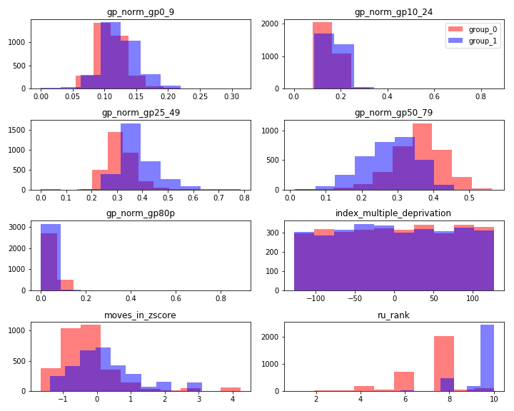
   The figure below shows the histograms of the confounders when the causal variable is the fraction of patients older than 80: blue bars denote the GPs with many elderly patients (group 1), red bars denote the GPs with fewer (group 0).

   

3. Perform the matching: we pair up GPs with many schools (those with causal variable = 1) with GPs with few schools (causal variable = 0). Here we compare two matching methods, described in the following sections: Mahalanobis Distance Matching and Propensity Score Matching.

4. Determine if the average loneliness of the matched GPs with many schools is significantly different from the loneliness of the matched GPs with few schools. Mathematically, this difference is quantified with the Average Treatment Effect: \({\rm ATE} = \sum_i^N ( y_i(1) - y_i(0) ) / N\), where \(y_i(1)\) is the value of the outcome variable (loneliness) of the GP with many schools in pair \(i\) and \(y_i(0)\) is the loneliness of the matched GP with few schools. A causal relationship is present if the ATE is significantly different from zero according to the t-test.

Here are the descriptions of the matching algorithms we considered.

Mahalanobis Distance Matching

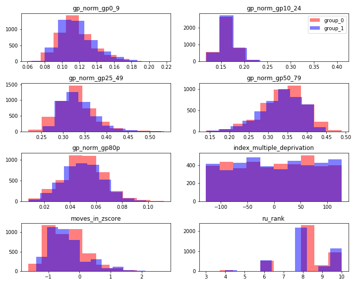
Mahalanobis Distance Matching is a popular kind of Nearest Neighbour Matching, which is one of the most intuitive matching methods. In Nearest Neighbour Matching a distance function is defined in the space of the covariates and each unit with causal variable = 1 is matched with the closest unit with causal variable = 0. In Mahalanobis Distance Matching the Mahalanobis distance is used, which is defined as \(d^{\rm MDM}_{ij} = \sqrt{(x_i -x_j)^T S^{-1} (x_i -x_j)}\), where \(x_i\) is the covariate vector of GP \(i\) and \(S\) is the covariance matrix. If the distance is larger than a predefined threshold, called caliper, the match quality is considered poor and we discard the pair. For MDM we set the caliper at \(1\) in order to exclude matched pairs with distances larger than the median. The figure below shows an example of Mahalanobis Distance Matching when the causal variable is the fraction of patients who are older than 80.

Propensity Score Matching

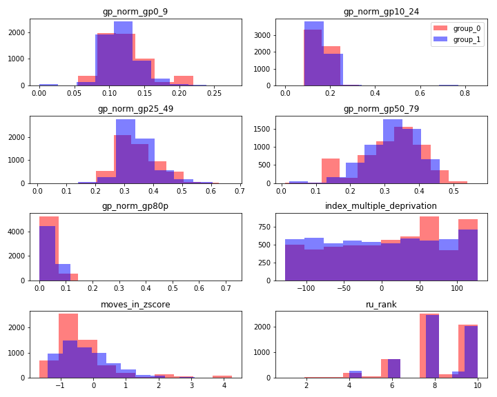
In Propensity Score Matching [2] GPs are matched according to a single variable, the propensity score \(\pi\), which represents the probability that a GP would have causal variable equal to 1, given the covariates. The propensity score is computed using a probabilistic model (here we consider logistic regression) to infer the value of the causal variable given the covariates. Once the propensity score of each GP has been estimated, we use Nearest Neighbour Matching to pair each GP with causal variable equal to 1 to the GP causal variable equal to 0 that has the closest propensity score. For MDM we set the caliper at \(0.005\) in order to exclude matched pairs with large distances. The figure below shows an example of Propensity Score Matching when the causal variable is the fraction of patients who are older than 80.

Quality of matching (Imbalance)

The validity of inference drawn using matching methods depends on the quality of the matching, namely if we were able to find enough pairs of GPs with different values of causal variable and very similar covariates. To assess the goodness of the matching we can compare the distributions of covariates for the two elements of the pairs and measure their distance: high distance, also known as imbalance, means the matching is far from a perfect matching where each GP is paired with a GP with exactly the same covariate values.
One measure of imbalance is the average distance in the covariate space between the GPs in each pair: \[ I = \frac{1}{n}\sum_{c=1}^n \frac{|\delta_c|}{\sigma_c} \] where \(\delta_c\) is the sum of the absolute standardised difference of all covariates between the two groups: \(c\) in group 1 and group 0 and \(\sigma_c\) is the standard deviation of covariate \(c\) across all groups.

Results

Here are the causal variables we consider:

• Percentage of patients younger than 25
• Percentage of patients older than 80
• Number of nearby schools (z-score)
• Multiple deprivation index
• Incoming migrations to the local authority of the GP (z-score)
• Rural-urban classification

These are the statistics we measure:

• Mean difference (ATE) of the outcome variable (loneliness score) between group 1 and group 0.
• t-test for the equivalence of means between the two groups, with two-tailed p-value rounded at four decimal places (a star denotes significance at 0.05).
• Imbalance \(I\) (absolute standardised difference).

Percentage of patients younger than 25

• Before matching, the fraction of patients between the age of 10 and 24 has a negative ATE (Mean difference) significantly different from zero, which means that GPs with young patients are less lonely.
• After matching, the ATE is still negative and significant, confirming that the percentage of young people has an impact on the loneliness score of a GP.

Percentage of patients older than 80

• Before matching, the fraction of patients older than 80 has a positive ATE (Mean difference) significantly different from zero, which means that GPs with older patients are more lonely.
• After matching, the ATE is still positive and significant, confirming that the percentage of elderly people has an impact on the loneliness score of a GP.

Multiple deprivation index

• Before matching, the index of multiple deprivation the ATE (Mean difference) is not significantly different from zero, which means that deprivation has no impact on loneliness.
• After matching, the ATE is not significantly different from zero, confirming that deprivation has no impact on the loneliness score of a GP.

Incoming migrations to the local authority of the GP (z-score)

• Before matching, the number of incoming migrations has a negative ATE (Mean difference) significantly different from zero, which means that GPs in areas with many incoming movers are less lonely.
• After matching, the ATE is no longer significant for both matching methods, suggesting that incoming migration has no impact on the loneliness score of a GP.

Number of nearby schools (z-score)

• Before matching, the number of schools nearby a GP has a negative ATE (Mean difference) significantly different from zero, which means that GPs in areas with many schools are less lonely.
• After matching, the ATE is still significant for both matching methods, but with opposite ATEs: positive for PSM and negative for MDM. This contradictory result does not allow us to draw a conclusion regarding the effect of the number of schools on the loneliness score of an area.

Rural-urban classification

• Before matching, the level of urbanisation has a negative ATE (Mean difference) significantly different from zero, which means that GPs in urban areas are less lonely.
• After matching, the ATE is still negative and significant, confirming that the level of urbanisation has an impact on the loneliness score of a GP.

Conclusions

The matching technique showed us that simple statistical analysis of group differences can lead to misleading conclusions regarding the influence of some variables on the outcome variable (e.g. incoming migrants).

This approach, however, has several limitations. First, it is based on assumptions that are difficult to test. To correctly estimate the Average Treatment Effect two assumptions must hold when performing the matching:

1. there shouldn’t be unmeasured confounders, i.e. we should consider all variables that can influence both the causal and the outcome variables,
2. we should not consider variables that are influenced by the causal variable.

The first assumption is very hard to verify, given that generally we cannot know all the variables that may have an influence on the variables under consideration. The second assumption is also difficult to test in the present case for the same reason, as it is not clear what control variables could be influenced by the causal variable.

Even if the assumptions necessary to establish causal relationship are not tested, matching can still allow to discover more meaningful relationship between variables in observational studies because it enables to make meaningful comparisons between similar units, as opposed to simple correlation studies.

References

[1] Stuart, E. A. Matching methods for causal inference: A review and a look forward. Statistical science: a review journal of the Institute of Mathematical Statistics25, 1 [2010].
[2] Rosenbaum, P. R. & Rubin, D. B. The central role of the propensity score in observational studies for causal effects. Biometrika70, 41–55 [1983].